Simulation of a four-bar linkage
When I was in college, I took a course in engineering dynamics, and as part of a final project, I had to submit a simulation of some mechanical system. Due to the plethora of different systems that are possible to simulate, it became difficult to select something in particular. After some deliberation and some counseling, I settled on a four-bar linkage as a system to simulate. A four-bar linkage is a classic and widely used mechanism that consists of four bars that are connected to each other. The connections between the bars are rotary hinges, meaning that each bar can rotate relative to the other in the sequence in which they are connected.
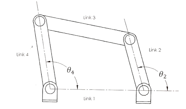
The mechanism has four bars with four joints
The complexity in this mechanism stems from the fact that the bars can be of different lengths, and that depending on which bars are held fixed in space, the motion of the mechanism changes. For example, if we hold one of the bars fixed and rotate one of the adjacent bars, we can convert rotary motion into reciprocating motion. This type of relationship is the basis for mechanisms like crankshafts, which purposefully make this conversion between motion types. Another advantage of this mechanism is that the motion occurs in two dimensions which makes it a lot easier to simulate.

The lengths of the bars can greatly affect the motion
Note: The simulation was written in the Python language due to its flexibility. While I did not know it at the time, there was a significant difference between Python 2 and Python 3, and due to concerns over compatibility, the class chose to use Python 2.
Before writing the simulation, it was necessary to first analyze the kinematics of the mechanism. It was quickly noticed that by keeping one of the members fixed, the kinematics of the mechanism reduced to a single degree freedom. This meant that through one variable, the rest of the motion of the mechanism could be determined through trigonometry. Since we also had to solve the dynamics of the system, it was the necessity to determine the equations of motion the bar that drove the mechanism. This was obtained by analyzing the mechanism with the D’Alembert’s principle of virtual work. In this method, the mechanism is assumed to undergo very small deflections, such that if we analyze these small deflections at the joints of each bar, each joint will be associated with a small force that induces a certain amount of work. By adding each amount of work, and by also taking into account the work due to accelerating each bar, it’s possible to generate an equation which dictates the entire dynamics of the system. Moreover, since the kinematics of the mechanism were ultimately determined by a single variable, it reduced the equations of motion to an ordinary differential equation.
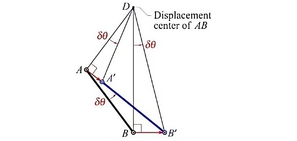
D'Alembert's method imagines small deflections
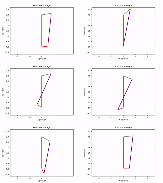
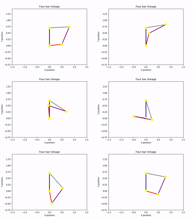
To visualize the results of the equation of motion, I created an animation of the mechanism. The solution to the ordinary differential equation could then be used to control the angle of the input bar during the animation. This was accomplished using the Canvas elements of the Matplotlib library. I created a drawing of the mechanism composed of line segments that joined at their vertices. These elements were animated with respect to a time variable, spanning from zero to an arbitrary future time. By knowing how one of the rods of the mechanism moved over time, I was able to create a complete animation. Thankfully, this information became available after solving the equation of motion. The output of the program was an animation of the mechanism rotating under the absence of damping forces. The lengths of the bars could be changed at the start of the program, as could the mass of the driving and driven bars. For simplicity, the intermediate bar acting as a conrod was assumed to be massless. Other inputs included the initial angular velocity of the rotating bar and a constant external torque acting on that bar. Here are some examples of the script’s output:
Animations generated by the simulation script
To gain a better understanding of how the simulation works, along with the details of the equations of motion and the animation itself, see the report which was written for this project:
See: Simulation of a four-bar linkage | Report
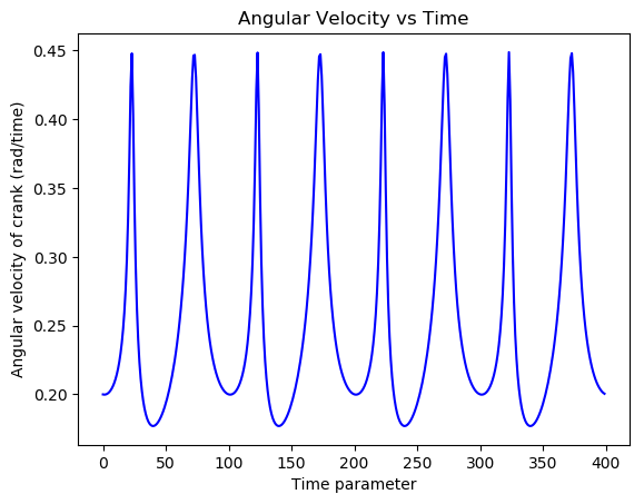
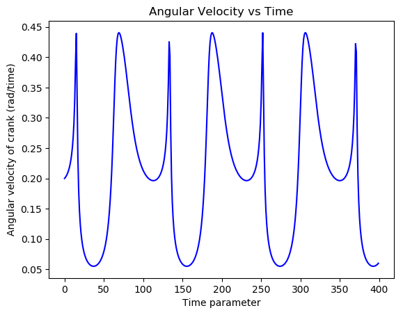
Analyzing the results of the simulation was interesting. It was evident that the mass of the bars played a significant role in the resulting motion. When one of the bars in the system was light and another was heavy, if the light bar completed a full revolution, the motion of the entire system became very jagged; there was considerable variation in the angular velocity of the rotating member. In contrast, when the rotating bar was much heavier compared to the other bars, the angular velocity varied much less throughout the system. The rotating element moved with a steadier angular velocity, while the oscillating bars exhibited a smoother overall oscillation. This can be interpreted as an exchange of kinetic energy. When the rotating bar is heavy, most of the kinetic energy of the system is stored in this element, resulting in a roughly constant angular velocity. However, when the oscillating bars store most of the energy, there are periods when that energy needs to be imparted to the rotating member to conserve the energy of the system, as the oscillating bars may not be moving or reversing direction.
Angular velocity changed drastically with bar length and mass
Overall, I was very pleased with the simulation’s outcome. It taught me a lot about simplifying the equations of motion of a system and focusing on the energy of the system rather than on the individual forces acting on it. Prior knowledge of the motion of the involved bodies can greatly simplify the analysis of their dynamics. If we lack this information, we must solve for the effects of the forces acting on the system, leading to much more complicated equations.
Github repository
To run the project, simply download the repository and execute the “FourBarSimulation.py” file in the Python terminal. It will automatically generate a video of the animation, which will be saved in the same location as the .py file. The script will also generate a plot of the angular velocity of the driven rod with respect to time. See the following link: FourBarSimulation
