2D simulation of a tracked vehicle
As part of the project to develop an autonomous tracked robot, I created a small script to simulate the motion of such a vehicle in two dimensions. This would allow me to experiment with parameters that are more difficult to control in real life, such as the friction between the surface and the tracks, or the dimensions of the treads. At the core of the simulation was a model for friction. This is a complicated force with non-linear behavior. Therefore, the model had to be chosen carefully to accurately represent realistic behavior while also being simple enough to avoid high computational costs.
See: Autonomous Tracked Robot | Project Review
A good compromise was a modified model of Coulomb friction, wherein the force due to friction depended only on the sliding velocity of the rubbing surfaces. This is not entirely accurate, as in the Coulomb model (as well as in real life), static friction is a prevalent behavior. Under these conditions, the two rubbing surfaces do not slide relative to each other but adhere to one another, resulting in no sliding velocity between the two surfaces.
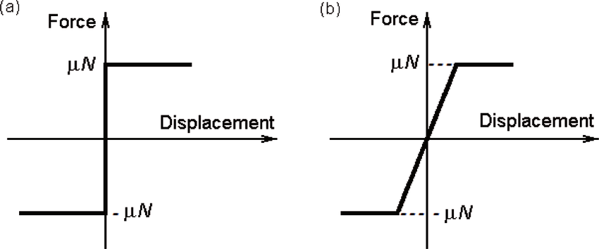
Friction can be approximated as a non-linear damping force
In the modified Coulomb model, the two surfaces will always move relative to each other. However, the velocity of this motion can be very small by making the slope of the friction with respect to velocity very steep. This means that even the most minute sliding velocity generates a large reaction force, which keeps the displacements of the two surfaces very low. In transient situations where friction only applies a force for short periods, these displacements can be small enough to be considered irrelevant. Therefore, the modified Coulomb model provides a reasonable approximation of the actual behavior of friction.
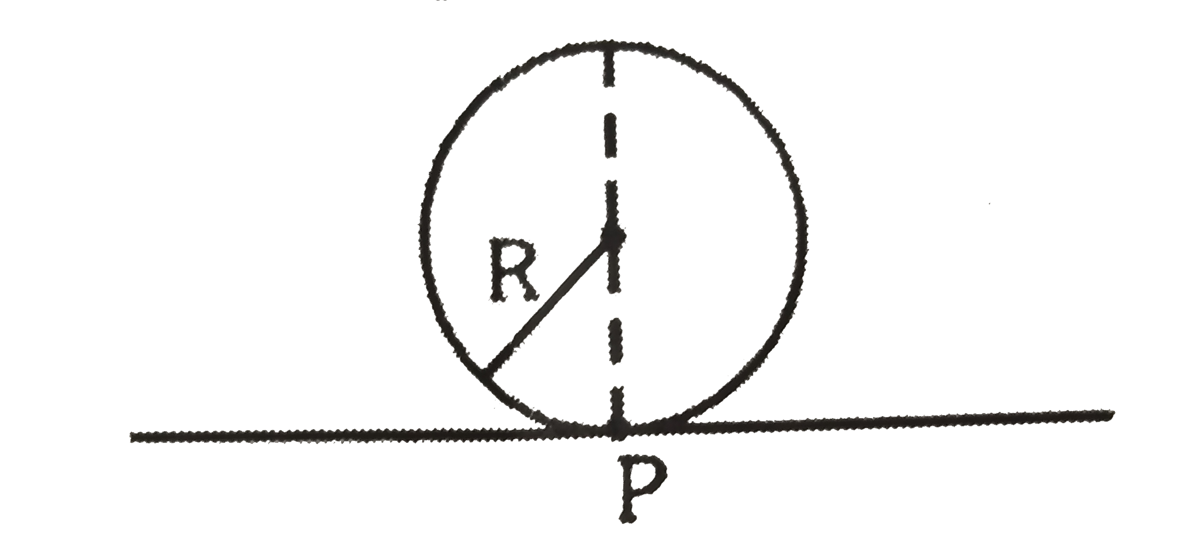
An ideal wheel rolls about a contact point
Unlike a wheeled vehicle that distributes its weight across small patches that can be assumed to be points of contact, a tracked vehicle distributes its weight over a much larger area. This means that the friction force is distributed across this area and not concentrated at a single point. If we subdivide the contact area into a grid of elements, the friction acting on these elements can be numerically integrated. These sums can then be used to estimate the net force and torque acting on an individual track. By repeating these computations for both tracks, we can combine these forces to obtain the net force acting on the vehicle.
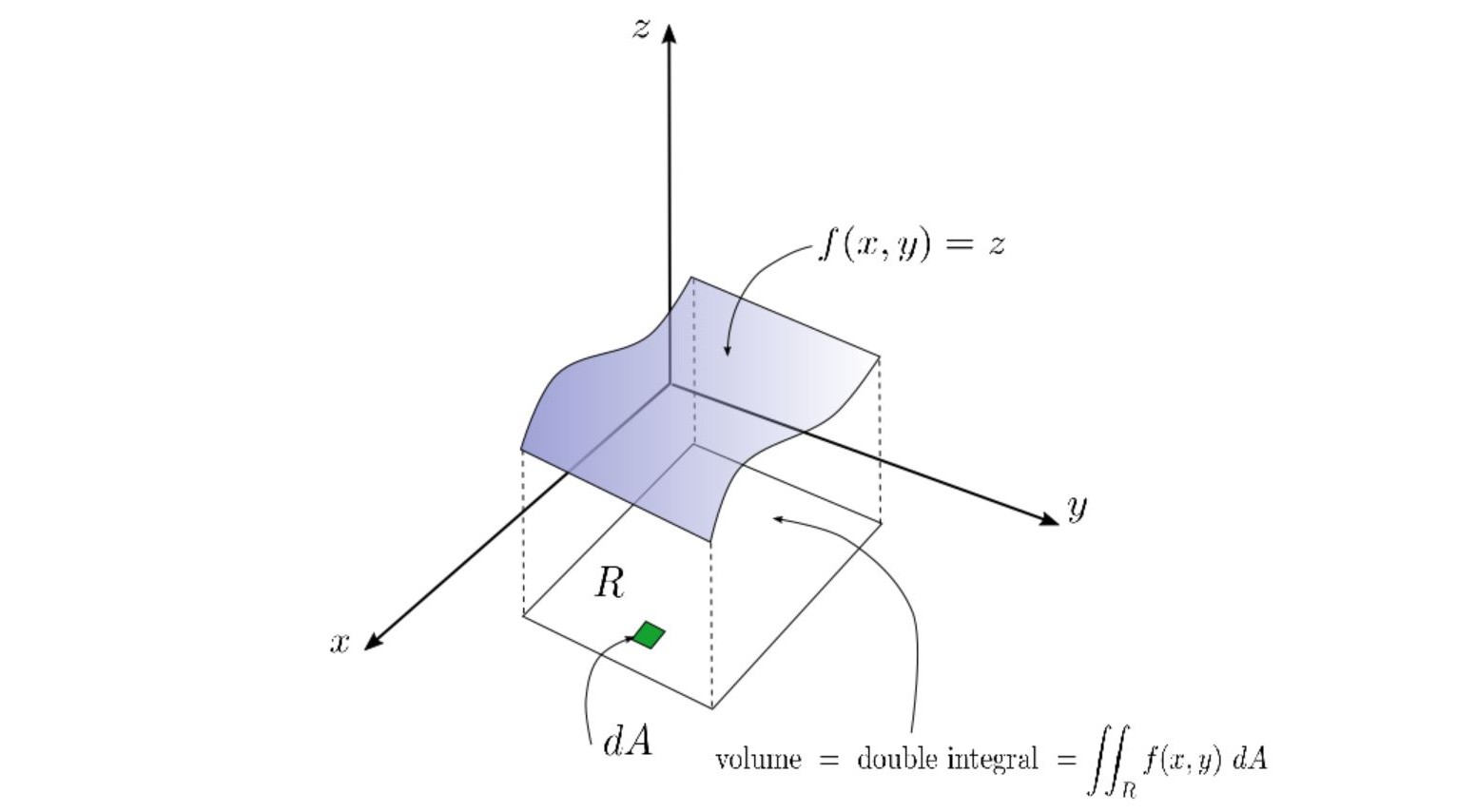
Friction had to be integrated across the surface area of the tracks
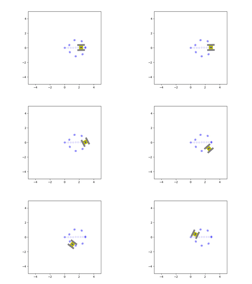
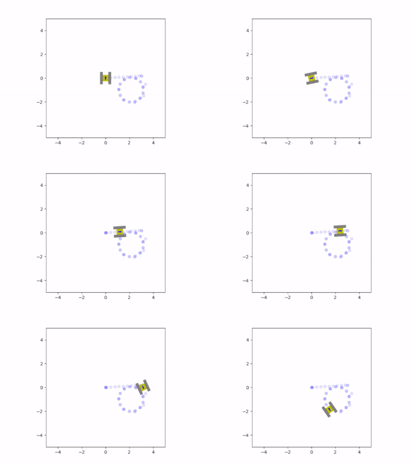
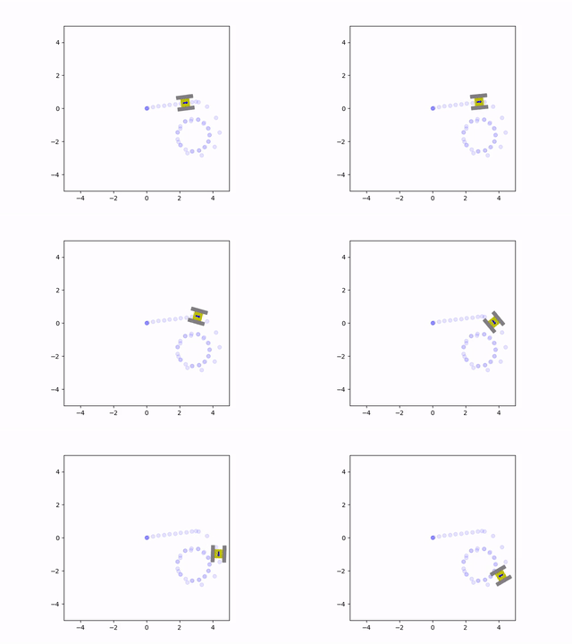
The net force and torque can be integrated twice to find the vehicle’s instantaneous velocity and position. These velocity estimates are fed back into the friction model to calculate a new iteration of velocity and position. This results in a system of ordinary differential equations that are solved simultaneously with each estimate for the net friction of the tracks. The solution to these equations provides the state of the vehicle, which consists of the rectangular coordinates of the center of the chassis and the angle of the vehicle with respect to the coordinate axes. The simulation was written in Python since it could easily perform these computations and animate the results. The Matplotlib library was used to create a small drawing of the vehicle and to illustrate the vehicle’s trajectory. This way, it was possible to view the vehicle’s path and how it moved in real time. This animation was displayed at the end of the program, once it completed the computations for the simulation. Here are some examples of the script’s output:
Friction greatly affected the trajectory of the vehicle during turns
When we analyze the motion of the vehicle, it’s clear that the friction coefficient played a significant role in its behavior, especially during turns. When the friction was very high, the tracks behaved similarly to a set of wheels located at the center of the tracks. However, if the friction was very low, the tracks would continuously slide during a turn. In the animations, it can be seen that there are sections of the tracks whose instantaneous velocity does not align with the velocity of the vehicle. The track that was farther from the instantaneous center of rotation would slide more than the inward-facing track. This is because the length of the chassis caused the outermost track to have a larger tangential velocity, leading to more local sliding.
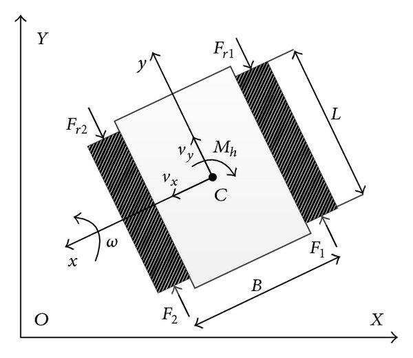
The simulation considered the position and angle of the vehicle
We can better understand this local sliding of the tracks by subdividing it into small sections and considering each one as a small wheel. Since a track does not have steering, all of the “wheels” must rotate in the same direction. However, because they are at different radial positions relative to the center of rotation, they will move in a direction that is not tangential to the radial direction. Therefore, each “wheel” lacks the equivalent of an Ackerman mechanism to provide the necessary steering to avoid sliding.
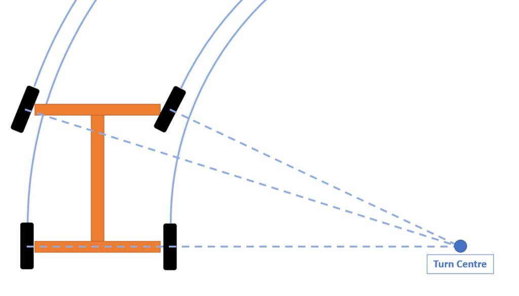
Wheels must rotate tangentially to the center of rotation to avoid sliding
These simulations clearly showed that a tracked vehicle would be incapable of using odometry to navigate. Tracks, especially under low-friction conditions, would slide too much to be used to measure displacements. This means that rotating the tracks did not always ensure the vehicle actually moved across the surface it was in contact with. In conclusion, this project taught me that simulating a vehicle before attempting to build it is extremely useful. It allows us to address unexpected behavior and gain a far better intuitive feel for what the vehicle will do. With this information, we can create closed-loop control systems that can compensate for these deficiencies or discard the vehicle as inadequate for our intended purposes.
Github Repository
The simulation can be run by executing the Python file included in the repository. The code will then perform the simulation based on a series of arbitrary control inputs, which can be modified by opening the script and rewriting the “inputVel” function. The animation will then be saved as a video next to the Python file. To download the file, see the following link: TrackVehicleSimulation
