Review | Tracked vehicle capable of following waypoints on a 3D surface
Introduction to Navigation
Arduinos are capable of many things, yet they are often berated as being underpowered and greatly inferior to other development board options. While from a computational standpoint this is true, they are nonetheless very capable devices when used intelligently. With clever and efficiently written code, it is amazing what they can accomplish on such limited computational resources. As an educational challenge, it is well worth our time to try and develop a complex program based on an Arduino, both for the technical aspects it teaches us and to grant us a degree of respect for what properly developed code can accomplish. A classic example of accomplishing great things with few resources is the flight computer of the Apollo landers:
The Apollo flew with the equivalent of an inexpensive microcontroller
In the case of an Arduino, these devices are often used to maintain the balance of small robots, or as the flight controller for remote-controlled aircraft. They serve this purpose very well but the Arduinos generally end up underutilized. We can extend their capabilities to the more complex task of navigation. It is one thing to merely keep a vehicle stable in space and quite another to precisely control its position and orientation. If we can accomplish precise state control then we can command the vehicle to follow a given trajectory, or move towards a given set of coordinates. These are much more complicated tasks that involve a higher level of abstraction and greatly depend on the nature of the vehicle in question. In the most general case, we must measure the state of a body that can rotate and translate in three directions to accomplish these tasks.
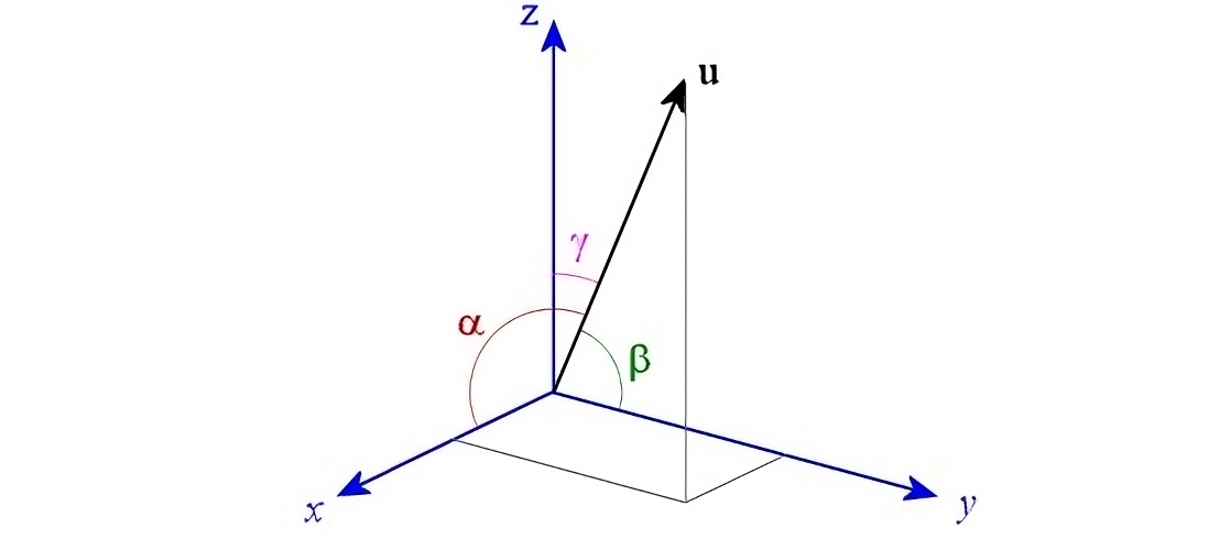
Under a Euclidean space, we can rotate and translate
We can further separate the problem of navigation into two sections: measuring the state of the body and precisely controlling said state. Once we can estimate what our vehicle is doing, we can take actions that affect its behavior. However, the nature of the vehicle in question greatly affects what we can alter. For example, in a car we can only change its forward and backward velocity and the direction it steers in. We cannot change its orientation with respect to gravity nor its side-to-side velocity. By comparison, there are variables that we can change (albeit with some restrictions) in a vehicle like a helicopter. This machine is capable of rotating about all axes and can translate in any direction, along with being able to rise and fall vertically.
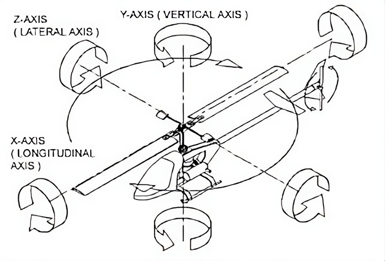
Not all vehicles have the same degrees of freedom
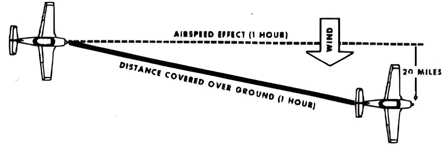
Given the intercoupled nature between the type of control we can obtain from a vehicle and the way it works, the more general component of navigation is measuring the state. This alone is not a simple problem and will depend greatly on the type of sensors we have available. In absence of the direct measurement of a variable, we must infer the state through a model that depends on related information. An example of such an inference is the process of dead reckoning. In this situation, we use the acceleration of a body to estimate its velocity. We have no direct knowledge of the velocity and therefore cannot determine whether it is true, but it is better than no information at all.
It’s not unusual for wheeled ground vehicles to estimate their position using the method of odometry. This involves counting the number of rotations of the wheels to determine how far the vehicle has displaced laterally and how much it has rotated. By combining this information, it’s possible to calculate the two-dimensional position of the vehicle by assuming it is moving across a flat plane. Since the actual position of the vehicle is never measured, this approach is a variant of dead reckoning that does not use velocity and time to determine position, but rather the assumption that a wheel in contact with a surface will not slide across said surface but roll over it. An ideal rolling wheel will only move forward if it has rotated a certain amount. The principal advantage of this method is the simplicity of the required calculations and sensors. A set of rotary encoders is enough to determine the rotation of the vehicle’s wheels and no other sensors are needed.
Odometry is a simple way to estimate position in the short term
Given that odometry has a tendency to diverge over time, it does a relatively poor job at determining the heading of a vehicle across any significant movement. Even small errors in displacement will get amplified when calculating the position, as any error in the heading gets amplified the farther the vehicle moves. We can clearly see this behavior when we compare odometry to gyrodometry. In the latter case the direction of the vehicle is measured through a gyroscope. These measurements are much more accurate than anything involving the wheels. As a consequence the position estimate in the long term is far better. The wheel displacement is used only to determine translation and the gyroscope handles the heading independently. When we compare both methods to one another, it’s clear gyrodometry is superior:
Gyrodometry improves upon odometry by using a gyroscope
Whilst gyrodometry is a better way of estimating the position of a wheeled vehicle, it is not without fault. The position is still being calculated by integrating many small individual measurements, and this will accumulate error over time. Moreover, this error also applies to the gyroscope, as the heading it holds as “zero” will drift with time unless it is routinely corrected. Therefore, gyrodometry still represents a form of dead reckoning that diverges relatively slowly compared to less accurate methods. Ultimately, if we do not have a way of directly measuring the position of the vehicle through a sensor (such that it does not accumulate errors over time), we will have no way to ensure the accuracy of our estimate in the long run. If we do have some way to verify our actual position, we can update our estimated position with something like a Kalman filter when we receive new data. We can see this update process in the following video:
A Kalman filter can estimate the state when there are no new measurements
By paying attention to the motion of the boxes, we can see that the measurements only appear sporadically and are not obtained in real time. The filter makes up for this deficiency by “filling in” the gaps between the measurements through an estimate of where it thinks the new measurement will take place. Essentially, the filter “mixes” the estimated position (which is updated much more quickly) with the measurements (which update slowly) to provide a “filtered” output. In the case of a wheeled robot, we can employ an additional sensor to provide a low-frequency but accurate measurement of position and supplement the time between measurements with gyrodometry.
Note: I highly recommend going over this Python script that simulates a 1-dimensional Kalman filter. It’s plain to see how the estimate “smooths” the infrequent measurement pulses.
It is clear that determining the position and orientation of a robot can quickly become very complicated depending on how demanding our requirements are. There exists a direct interconnection between the accuracy of our estimation and the types of sensors we have. Some sensors allow us to indirectly measure the state through an estimate, while others can directly measure the data without inferrence. Whatever the case, there is no mathematical wizardry that will prevent us from measuring something about the robot. From there on, it’s the measurement itself that determines how accurately we can infer other state variables.
Motivation for the Project
All of this discussion of navigation and how it may be implemented stems from my personal interest in a competition I learned about during college. On my campus, there was a team of students developing an autonomous excavator for the NASA Lunarbotics Challenge. The gist of the competition was to develop a robot that could excavate lunar regolith and transport it back to a rendezvous point. It had to accomplish this task autonomously without human assistance. The robot would have to go back and forth between the excavation point and its drop-off location multiple times, while also doing it as quickly as possible to win the competition.
This is an example of a Lunarbotics robot
In my case, I became interested in the navigation part of this challenge as I knew something about Arduino and this felt like a good way to expand my knowledge. Since the robot was assumed to operate on the moon, one of the restrictions imposed on it was that it could not depend on navigation systems that are used on Earth (like GPS and magnetometers). The entire navigation system had to depend on the robot itself with no external assistance. This is similar to how animals operate, in that they are closed systems that depend only on internal computations to navigate. Even “unintelligent” animals like small insects are capable of complex spatial localization. Honey bees are a fantastic example of what insects can accomplish with their very small brains:
Honey bees can fly to distant flowers and then return to their hive
This example from nature was very inspirational, as it meant that it was not unreasonable to use a limited device like an Arduino as a platform to develop a navigation system. Animals require far more effective navigation systems to locate food and survive, but the lunarbotics robot did not have such demands. It only needed to move towards a mining location and return to its original position. With this in mind, I felt confident that a small prototype based on an Arduino could be used to develop a navigation system that could be ported to the larger robot. Since the robot (which had already been manufactured) used treads to move over sand, it meant the prototype had to use this type of locomotion to effectively capture the dynamics of the larger vehicle. Obviously, it would not capture all of the dynamics, but it would still be much better than using a wheeled platform whose behavior differs significantly from a tracked vehicle.
Vehicle Dynamics
To better understand the dynamics and characteristics of tracked vehicles, I wrote a Python script that performed a simple 2-dimensional simulation. In this simulation, the vehicle was exposed to arbitrary control inputs that made the treads move at different speeds. This way one could observe how the vehicle would react to maneuvers like turning at speed and rotating about its own axis, or even external factors like changes in friction between the treads and the underlying surface. The most difficult part of the simulation was modeling the treads, as these are area contact devices rather than point contact devices like wheels. As a consequence, the force from the treads had to be obtained through the definite double integral of the friction across each track. This meant one had to subdivide the tracks into multiple small contact patches then integrate the friction force of each patch over the entire contact area.
See: 2D simulation of a tracked robot | Article and code
Through this analysis, it became clear that treads do not operate like wheels and constantly slide when the vehicle is turning. We can observe this by watching a tank rotate in place on a soft surface. Parts of the tread that are farther away from the center of the vehicle move with a tangential velocity, and this causes them to slide sideways as the vehicle rotates. This sliding motion occurs to every section of the tread, so even during small rotations of the chasis, the treads will be sliding and not rolling.
The trails left by the treads highlight how the treads slide across the surface
We can further observe this behavior through an animation generated by the simulation. Like in the above video, we also observe this strong sliding motion during turns. This lateral sliding gets worse as the friction between the tracks and the surface decreases, meaning that under conditions of low traction, the treads will be sliding almost all of the time.
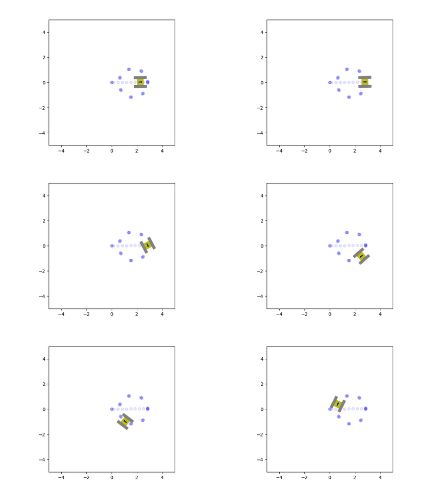
The trails left by the treads highlight how they slide across the surface
From the perspective of navigation, these dynamics are very detrimental as it means we cannot depend on odometry to provide accurate measurements of position, both in the short term and especially in the long term. This is because rotating the treads will not always guarantee a displacement of the vehicle. Therefore, at a minimum, we are forced to use gyrodometry to obtain somewhat reasonable navigation, and even then, its accuracy will depend greatly on the surface the vehicle is moving over. If we wish to obtain more consistent position estimates regardless of the properties of the surface, we must use additional sensors that can measure displacement independent of the motion of the treads.
Inertial Measurement
A simple enhancement is to make use of the accelerometer that is often bundled with gyroscopes as part of an inertial measurement unit. While we cannot measure velocity directly with this device, we can still integrate the acceleration to obtain an estimate of velocity. This is a complicated problem as we must take into account the rotation of our acceleration with respect to some reference frame. Therefore, we must keep track of our heading via the gyroscope to then properly integrate the acceleration about a fixed coordinate frame. These coupled dynamics can be obtained through a quaternion that encodes the orientation measured by the gyroscope.
Direct integration of an accelerometer leads to drift
Short-term position can be determined with an accelerometer by filtering the raw signal
Despite the hurdles that double integration presents, I was able to obtain acceptable velocity and position estimates through an accelerometer after many attempts. The solution came in the form of a modified version of the Kalman filter implemented in this Arduino library. In this filter, we have a variable with unknown behavior that has a known standard deviation. Any values of the variable that are within this error band, relative to a long-term average of the variable, will be suppressed. The end result is that the filter reacts slowly to small changes in the input variable and reacts quickly to large changes. This works well for integrating acceleration as we can suppress small variations in the acceleration to avoid integration drift, yet we still consider large accelerations to determine the velocity. We can find more details about the acceleration filter developed for this project in the following article:
See: IMU Filter based on a quaternion | Stable double integration
Real-time Dynamic Vehicle Model
One of the benefits of developing the double integration algorithm was the resulting information it generated about the vehicle. Prime among these was the establishment of a coordinate frame embedded in the heading measurement. Since we had defined a set of rectangular coordinates to measure the attitude from, we could use these coordinates to construct a 3-dimensional model of the vehicle based on the rotation of the tracks. Moreover, we could take into account friction and the sliding of the tracks to better estimate the position of the vehicle. This is essentially a more accurate way of performing odometry by considering a dynamic model that takes into account the forces acting on the vehicle, rather than assuming a specific set of arbitrary motions as odometry does (which is a kinematic model).
At the center of this improved dynamic model is a mathematical model for friction. Just by itself, modelling friction is a complicated topic, but if we consider a simplified model of friction, we can obtain usable results without much computational effort. A simple approximation is Coulomb friction. It defines friction as a function of the normal force acting on a body and separates it into two effects: static friction and dynamic friction. The transition between these two states is discontinuous with respect to sliding velocity, so it is not well-suited for integration using numerical methods. To circumvent this issue, we can define an approximation to Coulomb friction that is continuous with sliding velocity. See: Multi-Body Dynamics, B.3.1 Compliant Contact Models.
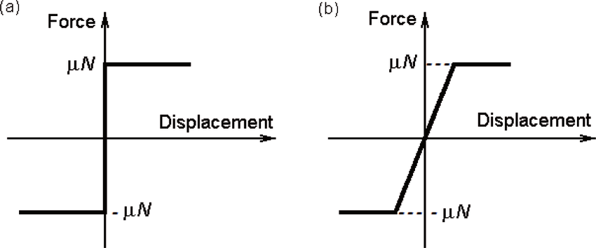
Friction can be approximated as a non-linear damping force
The continuous friction model should ideally have a very large slope when the sliding velocity is very small. This will allow us to better approximate static friction as it will keep the sliding velocities in this range very small (when ideally there should not be any). However, the need for a large force-velocity slope means we are in the presence of a stiff differential equation which is numerically unstable. We must therefore use specialized numerical methods to solve for the velocity as a function of acceleration, as our friction model is very sensitive to minor changes in velocity.
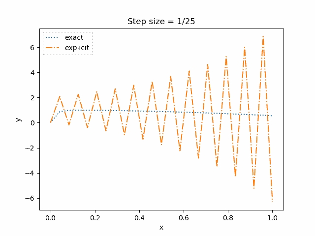
Some equations will cause a numerical solver to become unstable and diverge
To circumvent the numerical instability, I wrote a model that worked in two distinct phases: one phase measured the net lateral acceleration felt by the tracks, and if this value exceeded an estimate for the static friction coefficient (which would rapidly decrease if the vehicle rotated), it would be assumed that the vehicle did move laterally (velocity set to zero). However, if the static friction limit was below the current acceleration of the vehicle, then the continuous friction model would be used to determine the velocity through an explicit Runge-Kutta method. The coefficients of the method were carefully selected to be very stable for moderately stiff equations, meaning that while they would diverge if the equations were too stiff or if the time step between each iteration was too small, they were more stable than other choices of coefficients.
The end result was a model that would use as inputs the velocity of the tracks, along with the heading as measured by the gyroscope and the acceleration from the IMU, to determine the position of the robot. On a flat surface with high friction, it performed almost the same as odometry, but once the surface became inclined or if the traction was low, the model began to represent the lateral sliding that odometry did not capture. The cost of this additional accuracy was that the Arduino had to perform far more computations. Instead of just integrating some displacements, it now had to solve a set of ordinary differential equations in real time.
Optical Flow Sensors
As an additional fallback to further increase the robustness of the navigation of the robot, I chose to use optical flow sensors to directly measure the velocity. Unlike inertial estimates, which operate in the short term, and elaborate math models that only capture parts of the vehicle’s dynamics, a sensor that directly measures velocity is unambiguous. Unless something blocks the sensor, or if the conditions that allow it to measure velocity are no longer met, it is the most reliable authority on the state of the vehicle. Therefore, the addition of optical flow sensors to the robot is a good idea, and the other methods discussed above can be used to estimate position if the optical flow sensors cannot be used.
Optical flow sensors work by using a camera to take pictures of their environment, and each frame is compared to the previous one to determine whether a displacement has occured. There are many off-the-shelf sensors that perform these computations automatically. Possibly the most common application is inside optical mice, where the sensors are used to track motion without the use of any moving parts. It is for this reason that mice have a bright LED that shines on the surface they move across. It illuminates any small imperfections in the surface so that the camera in the sensor can detect motion.
In-depth explanation of how a computer mouse operates
A common and inexpensive optical flow sensor is the ADNS-3080. It is conveniently is sold as an independant module that can be easily connected to Arduinos. It communicates through the SPI protocol and there are a multitude of code examples that demonstrate how to do this. Unfortunately, when I purchased the modules there were no easily used libraries for this sensor. One had to write their own code to use the module, or modify a working example for their own particular use case. I disliked this approach, so I wrote a library that refactored some of the available working examples into a compact and easy-to-use interface. That way, I could connect multiple sensors to the Arduino without writing a lot of redundant code while avoiding any mistakes this could cause.
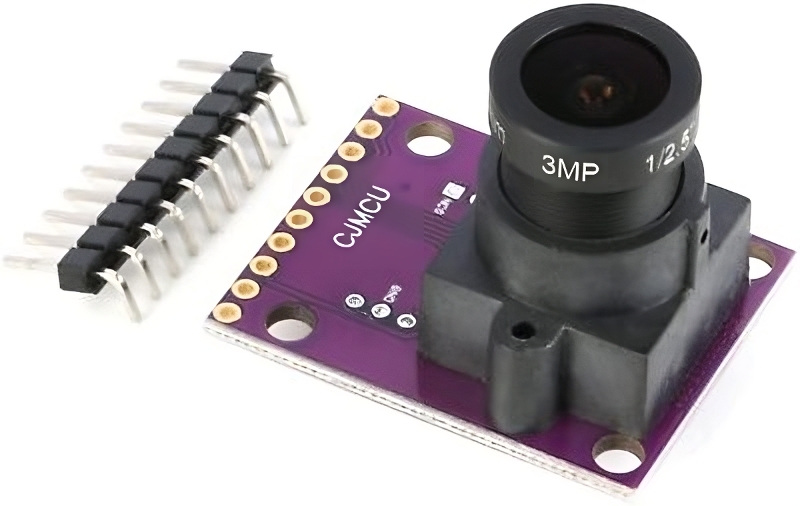
The ADNS-3080 is sold as a module
See: ADNS-3080 Mouse Sensor Library
I eventually settled on using two optical flow sensors as that was the minimum amount required to determine both translation and rotation. In the same way that odometry uses wheel rotation to determine displacements, we can replace these inferred displacements with actual measurements and still use the same equations. Therefore, we perform a kind of optical odometry that has much higher precision. We can find examples of this type of system in multiple papers. See the following:
PDF: High-Precision Robot Odometry Using an Array of Optical Mice
PDF: Optical Flow Based Odometry for Mobile Robots Supported by Multiple Sensors and Sensor Fusion
Because the optical flow sensors measure velocity instead of position, we must integrate their output to obtain position. This will induce drift, and in the long run, the estimated position will diverge from its actual value. However, since the velocity is directly measured, the rate at which the position will diverge will occur relatively slowly. While we will eventually have to calibrate our position estimate, it will not have to occur with that frequency. Moreover, if the divergence is slow enough, the error that is accumulated may not be large enough to matter in a given application. In the case of the mining robot, if the vehicle can complete multiple excavation and drop-off cycles, then it might not be necessary to recalibrate the position in order to achieve mission success.
Completed Robot
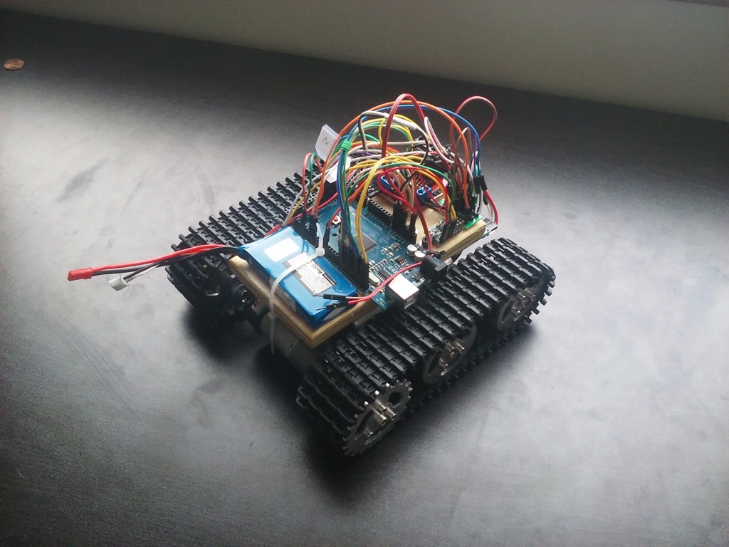
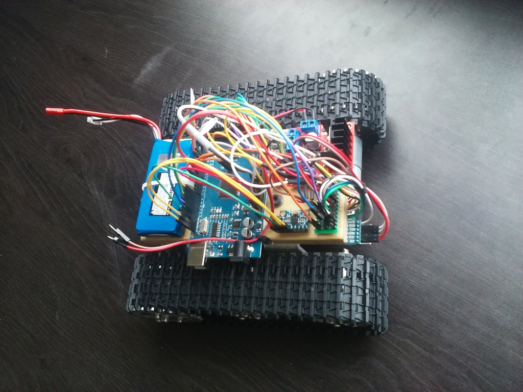
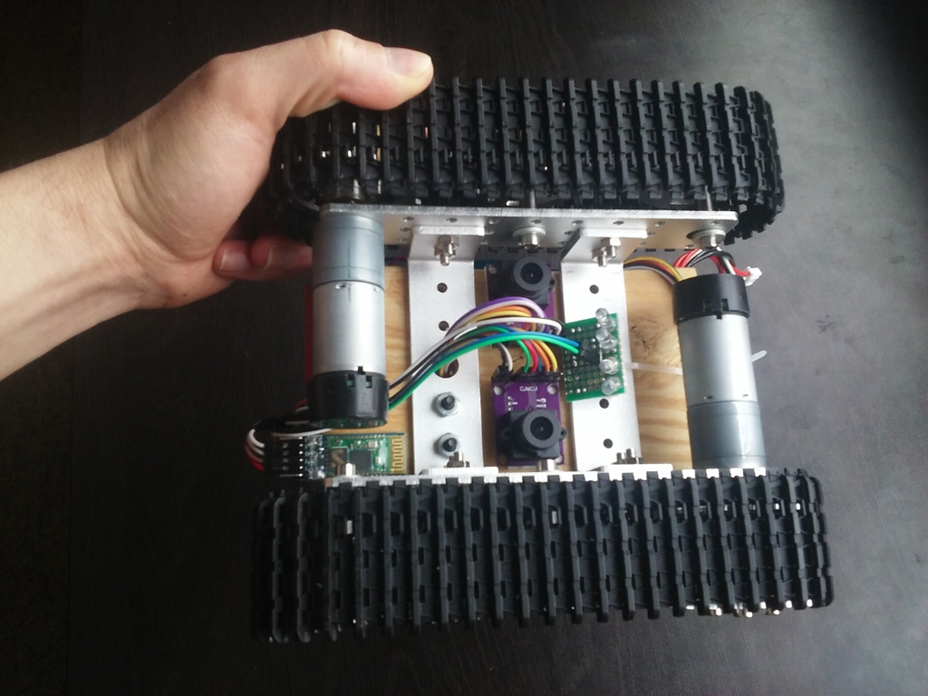
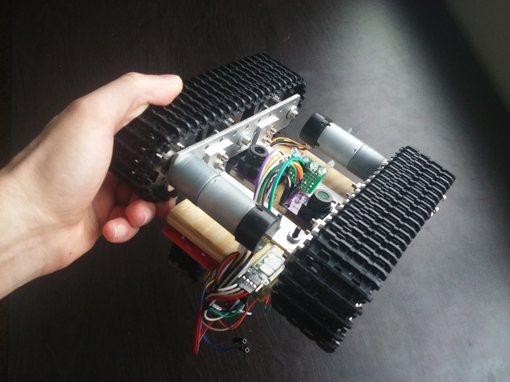
After the elements required to obtain the position of the robot were sufficiently developed, the actual physical robot was constructed. It consisted of the following components:
- An Arduino MEGA to connect to the multitude of sensors.
- Two ADNS-3080 optical flow sensors.
- An MPU-6050 IMU sensor to obtain angular velocity and acceleration.
- An L298N H-bridge module to drive a set of motors.
- An aluminum tank chassis with geared motors driving a set of tracks. Each motor had a set of rotary encoders.
- One 800 mAh, 2S Lithium-Polymer battery to drive the electronics and motors.
- A HC-05 Bluetooth Module for arduinos.
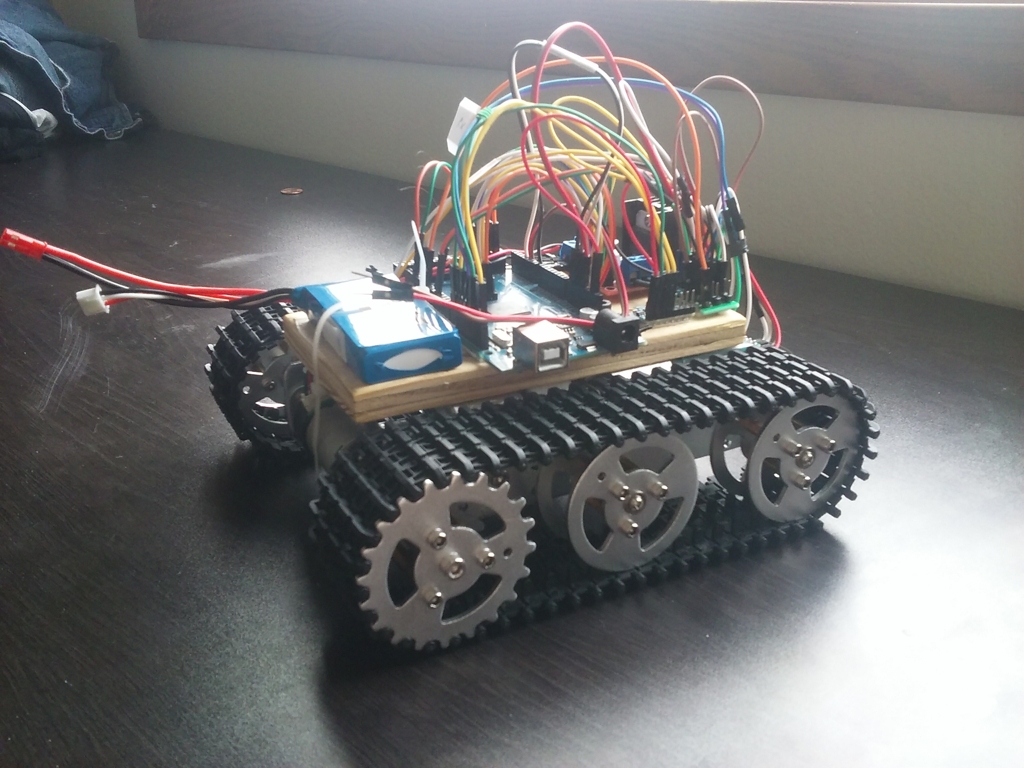
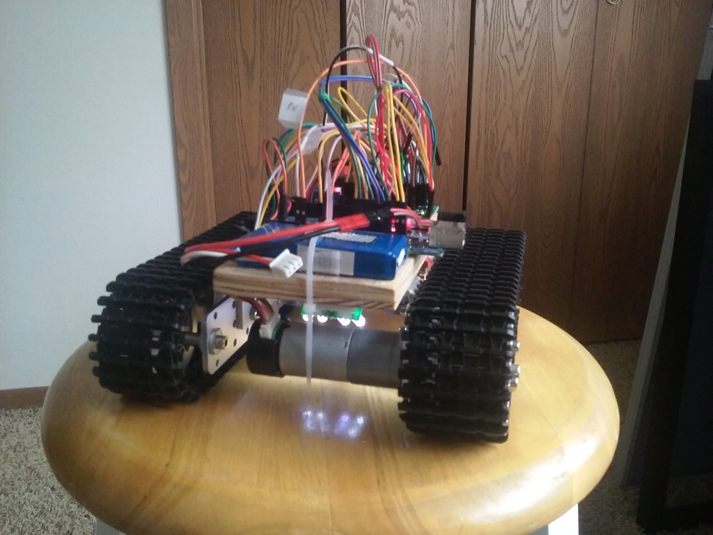
The assembled robot had the electronics exposed to easily modify any connections. This unfortunately meant the wiring was rather messy, but it allowed a necessary degree of flexibility as the prototype was being developed.
The tracked prototype was small and compact
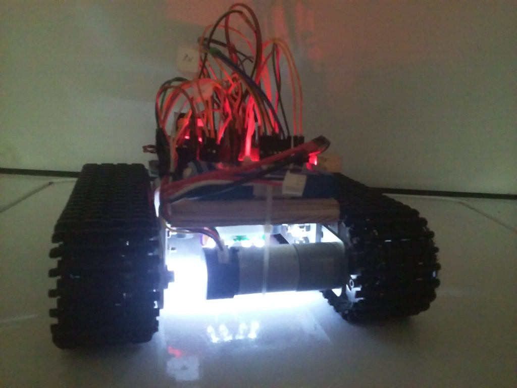
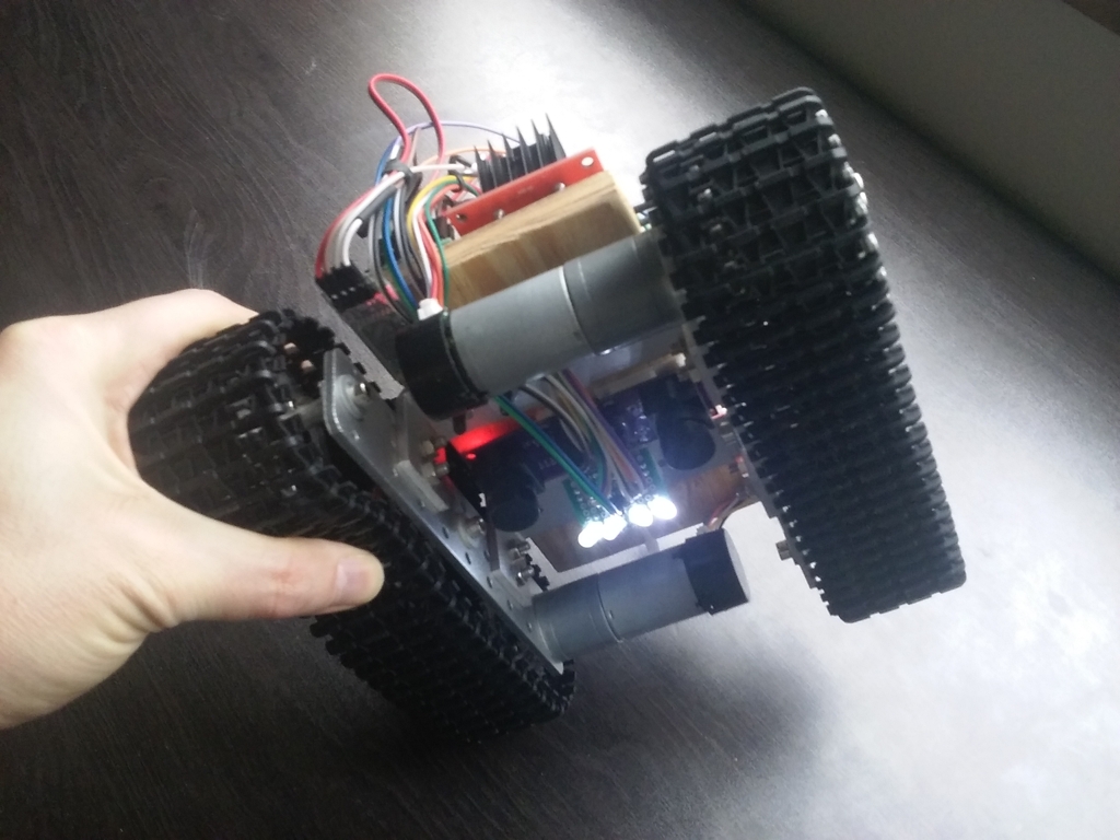
Once the optical flow sensors were mounted on the chassis, it became apparent that they required very intense light in order to operate properly. If the lighting was too dim, they would not measure any displacement. Therefore, a set of very bright LEDs were mounted beneath the robot to illuminate the surface the optical sensors were tracking. The color of the light also played an important role. At first, it was expected that red would be appropriate as that is generally what computer mice use. However, this did not work very well, and after some trial and error, I noticed that white light provided the most consistent motion tracking. The reason for this became evident once I observed the images generated by the cameras. White light provided the best contrast between surface features compared to blue, red, or yellow light.
Bright white LEDs were placed under the chassis to illuminate the ground
The position of the robot was estimated using all the methods mentioned above: the IMU was used to determine the heading of the robot and to estimate its short-term displacements with the accelerometer, and displacement was directly measured via the two optical flow sensors. All this data was then combined together via a completementary filter to obtain the position of the robot relative to an initial position. These position and orientation estimates were used to guide the vehicle to a specified coordinate using two PID controllers that set the required heading and lateral displacement.
Since the navigation algorithm considered the full 3-dimensional position of the robot, it was possible to precisely control it across uneven or inclined surfaces. These target coordinates were stored in a buffer that could be filled in real-time via a Bluetooth module. Once the vehicle lay within a given radius of a coordinate, the following coordinate in the buffer was made the new target destination. This process would continue indefinitely, and the vehicle would follow a closed path formed by the stored coordinates. The end result of all this behavior can be seen below:
The autonomous robot worked well with acceptable accuracy
It’s plain to see the robot worked pretty well. It did drift from its original position when asked to move over very large distances, but the error was rather small relative to its trajectory. For such a small and crude prototype, it demonstrated the feasibility of the position estimation methods discussed in this article. In particular, the successful use of an accelerometer to obtain position, even if in the short run, is especially noteworthy as this is considered a very difficult problem due to the rapid buildup of drift.
GitHub repository
The code for the project can be found in the following repository: TrackRobot
Note: Some versions of the code are written using older versions of the libraries it depends on. This is because the navigation code was being written at the same time as its
